Tracking the Trajectory of a mass using linear Kalman filter

The Kalman filter is an algorithm that estimates the state of a process from measured data. The word filter comes because of the estimations given for unknown variables, are more precise than noisy, inaccurate measurements taken from the environment. Kalman filter algorithm is a two stage process. The first stage (prediction) predicts the state of the system and the second stage (observation and update) updates the predicted state using the observed noisy measurements. In this post I explain an application of tracking the trajectory of a mass using linear Kalman filter. First let's have an idea about the kinematic model of a trajectory. 

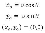Initial conditions

Now, let's look at the discrete linear Kalman filter equations.

Matlab code

 clear all; close all; clc;  
 N = 145; % no of iterations  
   
 %% parameters  
 v = 100; % initial velocity  
 T = 14.42096; % flight duration  
 deltaT = 0.1; % time slice  
 g = 9.80665;   
 theta = pi/4; % angle from the ground  
 F = [1 deltaT 0 0; 0 1 0 0; 0 0 1 deltaT; 0 0 0 1]; % state transition model  
 B = [0 0 0 0; 0 0 0 0; 0 0 1 0; 0 0 0 1]; % control input matrix  
 u = [0; 0; 0.5*(-g)*(deltaT^2); (-g)*deltaT]; % control vector  
 H = [1 0 0 0; 0 0 1 0]; % observation matrix  
 phat = eye(4); % initial predicted estimate covariance  
 Q = zeros(4); % process covariance  
 R = 0.2*eye(2); % measurement error covariance  
 xhat = [0; v*cos(theta); 200; v*sin(theta)]; % initial estimate  
 x_estimate = xhat;  
   
 %% system model  
 t = 0:deltaT:T;  
 x_sys = zeros(2,N);  
 x_sys(1,:) = v*cos(theta)*t ;  
 x_sys(2,:) = v*(sin(theta)*t)-(0.5*g*(t.^2));  
   
 %% noisy measurements  
 sigma = 25;  
 z = x_sys + sigma*randn(2,N);  
   
 %% kalman filter  
 for i=1:N  
   % prediction  
   x_pred = F*xhat + B*u; % project the state ahead  
   p_pred = F*phat*F' + Q; % project the error covariance  
     
   % observation and update  
   kalman_gain = (p_pred*H')/(H*p_pred*H'+R); % compute the Kalman gain  
   xhat = x_pred + kalman_gain*(z(:,i)-H*x_pred); % update estimate with measurement z  
   phat = (eye(4)-kalman_gain*H)*p_pred; % update error covariance   
   x_estimate = [x_estimate xhat]; %#ok[agrow] (to ignore array grow in loop warning)  
 end  
   
 %% plot results  
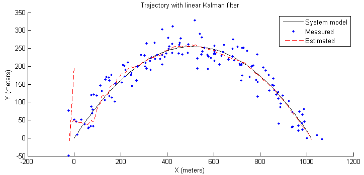
 figure; hold on;  
 plot(x_sys(1,:),x_sys(2,:),'k');  
 plot(z(1,:),z(2,:),'.b');  
 plot(x_estimate(1,:),x_estimate(3,:),'--r');  
   
 xlabel('X (meters)');  
 ylabel('Y (meters)');  
 title('Trajectory with linear Kalman filter');  
 legend('System model', 'Measured', 'Estimated');  

Simulation Results

 * You can download the matlab file from here.